Query Evaluation

This chapter is all about query evaluation. We've learned about the query languages and the operations available to the user, and we've learned how we store data on disk efficiently. In this chapter we learn how we unify these two concepts to efficiently answer complex questions about data through the query engine. We will learn about query optimization and query execution, as well as numerous techniques used in either step.

The Query Engine

Database systems exist to automate the work of describing how data should be stored and retrieved; as a result, they should also perform very well no matter how the user specifies the data they wish to have retrieved. As much as possible, the database should find the fastest possible way to retrieve a valid result for the user's query, no matter how convoluted the user's query was written.

The life of a query usually follows three steps:

Parsing: A parsing application transforms raw SQL into a logical query plan, typically represented by a tree.
Optimization: The logical query plan is transformed via a set of rules to an optimized query plan, which is then realized into a physical query plan, typically by comparing multiple candidate physical plans by their estimated cost.
Execution: The physical plan is executed by the database.

The first and last step aren't nearly as interesting as the second. First, some definitions. A logical query plan specifies the operations that the database should take to transform the data, but doesn't specify what specific algorithm or technique it should use. It is essentially a tree version of a SQL statement. A physical query plan on the other hand is a logical query plan that specifies exactly which algorithms it will use at each step. Query optimization, therefore, transforms a logical query plan into a (close to optimal) physical query plan. Simple, right?

Tnfortunately, it happens to be that query optimization is an incredibly hard problem, especially for larger queries. As we know from studying relational algebra, there are infinitely many equivalent query plans, and a potentially huge number of equivalent normalized query plans. Moreover, even if we were able to enumerate all possible query plans, deciding which one is best is difficult - there isn't a great way to know how long a query plan will take to execute without executing it.

We will first go over how a logical query plan can be manipulated to perform better without any knowledge outside of the query itself using rule-based optimization. Then, we will survey some of the more interesting algorithms that a query optimizer may be selecting from, as well as outline how their costs might be estimated in a cost-based optimizer.

Rule-Based Optimization

From relational algebra, we know that there are certain transformation we can apply to a query plan without altering it's final result. In fact, it turns out that there are a few of these transformations that will always result in faster execution times; we can call these transformation rules. Enumerating and applying these rules is the job of a rule-based optimizer. We will go over a few common rules.

Consider a query plan with the following substructure: $σ_{A_{c}} (A ⋈ B)$ . In English, we are processing a join between $A$ and $B$ , then filtering out the result viathe condition $A_{c}$ , defined over $A$ . It turns out that this substructure is equivalent to $σ_{A_{c}} (A) ⋈ B$ - intuitively, because we are only filtering based on attributes of $A$ , all matching rows of $A$ will be filtered out of the join result, and thus, we can simply filter them out before we apply the join. This clearly results in faster execution time, as the input to the join is smaller. In the best case, $A_{c}$ filters out all of the rows and the join doesn't have to happen at all! This optimization is called predicate pushdown because we push predicates through joins.

Consider a query plan with a complicated conjunctive condition in a filter, like: $σ_{c_{1} \land c_{2} \land c_{3}} (A)$ . We can instead apply the filters one after another in order, like so: $σ_{c_{1}} (σ_{c_{2}} (σ_{c_{3}} (A)))$ . We can commute these conjunctions in any order (do to commutativity of boolean operators) and choose the order that will leave us with the smallest relation as early as possible. The reason this may save some time is that it allows us to spend less time evaluating unnecessary parts of the predicate. However, if the predicate is simple, this optimization may only end up hurting our computation as we are usually disk- instead of cpu-bound. However, the inverse optimization is also valid, in case we want to combine multiple selections! This optimization is called cascading conjunctions.

Consider a query plan that only outputs column $c$ of a set of columns $C$ of a schema $S$ , without operating on any other columns. Then, instead of selecting all of the columns of $S$ , we can instead only select values in $c$ . In other words, we will add a projection after the selection to limit the amount of unused information flowing through our query. This optimization is called column filtering.

Many such rules can be dreamt up and used, and depending on slight changes in the data and execution model, different rules could be effective. Choices on whether to apply each rule once or many times or until convergence are up to the database designer.

Query Execution Algorithms

Now that we've reduced our logical query plan to a more optimized form, we'll need to decide how exactly we should execute it; that is, which algorithms we should ask our database engine to use to evaluate each step of the query plan. Indeed, for each operation we could be doing, multiple valid algorithms exist with different time and space complexities. We'll gloss over scans, then go over the canonical algorithms for joins (algorithms for selection boil down to using indexes when we can, and for the rest are not particularly interesting).

Scans

In order to actually have any data in memory to work with, we must first scan it from our tables. For the most part, we have two main choices: scan over the relevant blocks without an index, or rely on an index and do an index scan. While it might seem that an index scan is superior, depending on the query, different scanning approaches may be more suitable. For example, if a query is a restrictive range query over a nonprimary attribute with an index over it, then using that index might make sense; however, if it isn't a particularly restrictive range query, then using the secondary index might cause many unnecesary page evictions as we access pages out of order. Indeed, in this case it may be smarter to simply read all of the rows, then filter them out. Another consideration is sortedness; say we would like to apply a merge-join later; scanning in order might allow us to avoid a merge-sort later, which can save time. Optimizing for all these cases is difficult, and often left to a cost optimizer.

Loop Joins

The most basic join algorithm is the loop join! The loop join essentially works as follows:

for row s in S:
  for row t in T:
    if s.key == t.key:
      output(s, t)

This join is called the nested loop join. It might not immediately clear why, but this is probably the worst possible approach. Thinking about this in terms of block transfers, assuming the relation $T$ doesn't fit entirely in memory, we will have to transfer every block of $T$ into memory for every single row in $S$ . This is awful!

We can do a little better. Instead of going through each row in $S$ one after another, let's operate at the block level and try to process every row in each block in $S$ at a time:

for block b_s in S:
  for block b_t in T:
    for row s in b_s:
      for row t in b_t:
        if s.key == t.key:
          output(s, t)

This join is called the block nested loop join and is much better. We can do even better by choosing $S$ to be the smaller relation; if $S$ is small enough to fit entirely in memory (with at least one extra page frame left free), then we only have to scan through $T$ once! As we'll see, there are other, better techniques for joining than loop-based ones in general. However, when we only want to output a few rows (and thus can terminate early; see the LIMIT keyword), or in cases where one of our relations is sufficiently small, a block nested loop join is a great option.

Hash Joins

When performing a classic hash join algorithm on two tables, we have to find tuples that match on some key or value across both tables. To do so, the classic hash join creates a hash table index over the inner table, and then linearly scans the outer table, probing the inner table for corresponding values. However, due to the nature of hash functions, these tuples are distributed at random in the inner hash table. If the hash table is too large to reside entirely in memory, then we have to fetch data from disk at random, which greatly increases our disk I/O cost because pages will keep getting churned through our buffer cache. To illustrate this point, imagine that our inner table gets hashed into 100 buckets, and memory can only hold 8 buckets. For each tuple in the outer table, we are likely going to need to go to a different bucket. So, we end up doing one block transfer per element in the outer table; at this pace, we may as well have done a nested block loop join.

Luckily, the Grace hash join offers us a solution. Let's say we have two tables, denoted $L$ and $R$ . We'll say WLOG that $L$ is our outer relation. The Grace hash join will first extract the entirety of $L$ and $R$ into two hash tables using the same hash function, using each table's join key as the search key; concretely, if we were joining $L$ 's value on $R$ 's key, then we would create one hash table with all of $L$ 's tuples, hashed on their value, and another hash table with all of $R$ 's tuples, hashed on their key. Buckets are written out to disk to avoid running out of memory. Critically, the two hash tables are made to have the same global depth, even if this means expanding one table without splitting any buckets.

After partitioning our two relations and resizing our hash tables so that we have the same number of entries in our global index, we then load corresponding pairs of buckets into memory and match up pairs of tuples. Concretely, we load the ith bucket from $L$ and the ith bucket from $R$ , which should contain elements with the same hash on the join key. Since we used the same hash function, if there was a value in $L$ that matched with a value in $R$ , they would be in the same bucket pair, because otherwise, their hash keys must have been different, so they wouldn't have been in a bucket pair. We repeat this matching process for every pair of buckets until we have finished iterating through the buckets.

The main issue to worry about is duplicity; if we ever come across the same pair of buckets twice, we may end up outputting duplicate join results. This is possible if we were to use extendible hashing and weren't careful about our pointers. Thus, it is important to be sure that we never process the same pair of buckets twice; keeping track of which pairs of buckets we have seen will solve this problem.

Also notice that each pair of buckets has a disjoint result set (think about what it would mean if result sets weren't disjoint), indicating that there is room for parallelization. Clearly, this is a problem with many possible optimizations; we will explore in depth one such optimization through the use of a Bloom filter.

Bloom Filters

One inefficiency in a hash join is that you potentially have to iterate through an entire bucket to find a value. To do that for every search value is really expensive - if we could speed up our search time somehow, that would be a huge win! Unfortunately, maintaining a bucket ordering doesn't really make sense just for a one-time search, and building an index over such a small data structure is overkill.

Bloom filters are a lightweight solution to the sparse search problem. A Bloom filter is a probabilistic data structure that can tell us one of two things about an element: whether it is definitely not in a set, or possibly in a set. See a visual simulation of a bloom filter here.

A bloom filter has two parts: a bitset (essentially an array of $m$ bits) and a set of $n$ hashes (in this assignments, $n = 2$ ). When we insert an element into a set, we hash it $n$ times and take those values modulo $m$ - call these values $h_{i}$ . We then set each $h_{i}$ -th bit to 1 in our bitset. As a concrete example, let's say the string "hello" hashed to 3 and 5. Then, we would set the 3rd and 5th bit (0-indexed) to 1.

Next, when we want to check if a particular element is in the set, we hash it $n$ times and take those values module $m$ - call these values $h_{i}$ . Now, if at least one of the $h_{i}$ -th bits are 0, then we know for certain that the element in question is not in the set; if it were, then all of these bits would be 1. If they are all 1, then we know that it is possible that the element in question is in the set. But we can't say for sure that the element is present, since the bits may have been set by a combination of other elements that set all of those bits to 1. However, with a large enough bitset and enough hashes, we can avoid collisions as much as possible, making this a nearly constant-time check for inclusion.

Applying this to the Grace hash join, we will construct Bloom filters on each bucket of the inner relation, then during the probing step, first check to see if each value in the outer relation's $i$ -th bucket is definitely not in the Bloom filter. This will save us time, especially when joins return few tuples!

Sort Merge Join and External Sort

In the case that our input relations are sorted, we can use a sort merge join. A sort merge join essentially uses one pointer per relation, and runs through each relation outputting pairs that match on the join key. This join exploits the fact that, when joining over a sorted field, matching tuples will be in the same relative region of their respective sorted tables. Special case should be taken when there are duplicates, but this is an overall rather intuitive algorithm to describe and implement. The difficult part is sorting the relation.

If the relation isn't already sorted by primary key, then we have to do some work to sort it. Thankfully, the classic merge sort algorithm generalizes great to our setting, because we can treat each block like an array segment. However, instead of doing the entire search in memory, we write out intermediate sorted blocks. This algorithm is known as external sort. The algorithm proceeds as follows:

Sort each block in memory and write them out to disk. Each block is currently its own sorted chunk.
On iteration $k$ , read the first block of adjacent sorted chunks into memory and merge sort them, using a block-sized buffer. As this buffer fills up, write it out to a new chunk. Proceed for all chunks from iteration $k - 1$ .
Proceed until the whole table is sorted.

external

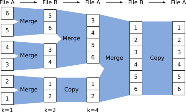
Notice that when we are on iteration $k$ , data from iteration $k - 2$ is now useless, we can get away with only using $2 N$ extra bytes of space if the original relation was stored using $N$ bytes. Notice also that this is a somewhat parallelizable task; indeed, it is often parallelized. Once we have a sorted relation we can apply sort merge join. Now that we've seen a plethora of join algorithms, it's time to see how the cost-based optimizer takes these candidate algorithms into account and decides on a physical query plan.

Cost-Based Optimization

To decide on a query plan, the optimizer repeatedly proposes a physical plan and estimates the runtime, or cost, of that physical plan until it reaches a point where it is satisfied. This is a delicate balancing act between finding a good physical plan and wasting time looking for a better physical plan; indeed, the query optimization problem is very difficult, and achieving optimality for large enough queries is often impossible. To see why, remember that joins are both commutative and associative; as a result of commutativity, for a query using $n$ tables there are at least $n!$ possible join orderings, and as a result of associativity, there are at least the $n$ -th Catalan number of possible join groupings. Combining these, plus the number of different join algorithms we could use yields a gargantuan number.

The optimizer can't compute cost without some statistics about the database. Most databases collect metadata about the size of their tables, the relative density and distribution of the data, and other metrics that may be useful in query planning. Indeed, these values can be very useful in estimating the time it will take for a join to run, and the size of the output of a join. With these values, the optimizer can recursively decide on estimates to compare between physical plans. The hardest challenge in optimizing queries is deciding on a join ordering, then on which join algorithms to use. Indeed, we would like for joins to result in smaller tables as soon as possible, but it is impossible to know the size of a join before executing is. However, using information about table sizing, we can get a decent estimate over which order to impose.

There are a few difficulties with this approach. First, once we start making estimates based on estimated values, our margin of error expands exponentially. Indeed, cost estimation is an incredibly inexact science, and often query plans execute much differently than expected. Moreover, because it is nearly impossible to explore the entire search space, deciding which plan to evaluate next is also a challenge. We leave further exploration of the realm of query optimization for another text.

Code Generation

At the end of the road, we've decided on a query plan, and for each relational node, an algorithm to use. Now, we will convert this query plan into executable code for our database engine to ingest and run. As this is more a concern for compiler-writers, we eschew a lengthy discussion of code generation.