Indexes
This chapter is all about indexing. Now that we have an idea of how data is stored in memory and on disk, we need to address another fundamental problem: efficient retrieval. We will learn about the kinds of indexes and in which cases we want to use them, and we will learn of two data structures that allow us to do efficient lookup and range querying: hash tables and B+Trees.
Indexing
Let's look at what happens if we take our data representation and try to answer a few questions on it without any indexing. If we want to return the row with id=12345, since we have not imposed any structure on our data so far, we have no choice but to scan all of the data blocks until we find our desires row(s). This takes time linear in the number of entries \(O(N)\), which is not very efficient. We can clearly do better!
Firstly, notice that we were searching for something by its id. Let's assume that all of our schemas have some attribute which is unique and orderable (e.g. a primary key). Then, let's impose that all of our data be stored sorted in primary key order. The idea is that, due to foreign key relations, we will likely be looking up by primary key rather often, so by sorting by it, we can employ tactics like binary search. Instead of scanning through every block now, we perform binary search over blocks until we find the record that we want. This is much better, in that we only have to peruse \(O(logN)\) blocks instead of \(O(N)\) of them.
However, notice that each block contained a lot of extra information that we didn't need to find our desired row. We already knew based on the first and last entry of each intermediate block we looked at whether or not our desired row was there. What if we could store this metadata about blocks somewhere else, so that we knew exactly which data block to read beforehand? This is the essense of a block.
Sparse and Dense Indexes
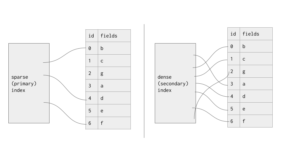
Nearly all database systems stores their data in primary key order. Building an index over this order is simple, and the nice part about it is that we don't even need to store the location of every tuple! This is because, as we've seen, as long as we know the range of values contained in each block, we know which block to read, after which a scan is cheap and easy (remember that the expensive operation here isn't a linear time scan over a particular block, but the disk read itself). As a result, primary key indexes are called sparse indexes, and they only store every few values in it. This is to save on space and make searching for values a little faster.
However, we aren't limited to building indexes over primary keys; we can build indexes over any attribute we like. Depending on what queries you expect from your users, a database operator might choose to build indexes over different attributes, and indexes can be built and destroyed over the lifetime of a database as needs change. However, building an index over any attribute raises a few problems. Firstly, we don't have the ordered property we had before, meaning we truly do need to store every value in the index. Thus, secondary key indexes are called dense indexes, since they referenc every value in the database. Secondly, we don't have the uniqueness property we had before, meaning we may have duplicate keys involved. This makes binary searching slightly more complicated, but is uncomplicated to handle. As a result of these two considerations, it may be clear that building an index over a secondary key is sometimes too costly to be worth it, as storing and maintaining it is a nontrivial task.
Now that we've seen the motivation and categorization of indexes, let's move into a few indexing methods.
Hash-based Indexing
Indexing based on hash tables are often used for quick "\(O(1)\)" lookup. As you'll see, not all of these schemes are necessarily constant for all operations, all the time, but their amortized cost is rather low. Hash-based indexing methods, however, do not support answering range queries, which our later tree-based indexing methods do.
For all of our hash-based indexing methods, we will need to choose a hash function \(H\). Ideally, this hash function is fast and uniform across the output space, meaning that keys will be uniformly distributed across the buckets. A non-cryptographic hash function such as xxhash or murmurhash will work just fine.
Static Hashing
The first indexing method we'll explore is called static hashing. In static hashing, we first choose a hash function \(H\), then a global modulus \(M\). A static hash table consists of a table and \(M\) buckets, where bucket \(i\) is denoted \(b_i\). On insertion of a row \(R\) with search key \(r_i\), we first compute \(H(r_i)\) and insert the location of \(R\) at the end of bucket \(b_{H(r_i) \mod M}\). On lookup of row \(R\), we do the same calculation, then scan through bucket \(b_{H(r_i) \mod M}\) until we find the entry, then access it in a data block. On deletion of a row \(R\), we do the same calculation, then scan through bucket \(b_{H(r_i) \mod M}\) until we find the entry, then delete it.
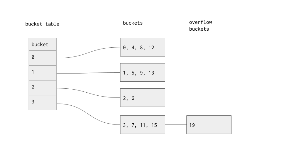
Indexes are stored on disk, just like data blocks, and the first question that should come to mind is how each indexing method is stored on disk. Each bucket is represented by it's own page. Once a bucket has too many entries to fit in one page, overflow pages are created to hold extra entries. This is clearly an issue; very quickly, if our value of \(M\) was too small, we will end up having to do linear scans through multiple overflow blocks, reducing our scheme to a linear search. This is no good, and is a primary reason why static hashing is never used in practice.
Extendible Hashing
Extendible hashing is a method of hashing that adapts as data is added. This is a direct upgrade from static hashing, which grows more and more inefficient as data is added to the system. The basic idea is that instead of allocating overflow blocks when a bucket gets too large, split the overflowing bucket into two buckets and double the size of your table (i.e. double your modulus value \(M\)).
An extendible hash table has two moving parts: the table and the buckets. The table is essentially an array of pointers to buckets. Each bucket has a local depth, denoted \(d_i\), which is the number of trailing bits that every element in that bucket has in common. The table also has a global depth, denoted \(d\), that is the maximum of the buckets' local depths. When we initialize it, the extendible hash table should look just like the static hash table with some extra bookkeeping.
On lookup of a row \(R\), the search key \(r_i\) is hashed, and then the table is used to determine the bucket that we should look at. The last \(d\) bits of the search key's hash are used as the key to the table, and then we do a linear scan over the bucket it points to.
On insertion of a row \(R\), the search key \(r_i\) is hashed, and then the table is used to determine the bucket that our new tuple should be in. The last \(d\) bits of the hash is used as the key to the hash table, after which we add the new tuple to the end of the bucket.
On deletion of a row \(R\), the search key \(r_i\) is hashed, and then the table is used to determine the bucket that our tuple should be in. The last \(d\) bits of the hash is used as the key to the hash table, after which we scan through the bucket and delete the entry we were looking for. Depending on your scheme, the other values may have to be moved over to fill the space it left. A good indexing scheme would use slotted pages to avoid this, for example. There are many ways to handle deletion, since we don't have to maintain any sort order on the bucket level.
Splitting
When a value is inserted into a hash table, one of two things can happen: either the bucket doesn't overflow, or the bucket does overflow. If it overflows, then we need to split our bucket. To split a bucket, we create a new bucket with the same search key as the bucket that overflowed, but with a "1" prepended to it. We then prepend a "0" to the original bucket's search key. As an example, if a bucket with a local depth of 3 and search key "101" splits, we would be left with two buckets, each of local depth 4 and with search keys "0101" and "1101" respectively. Then, we transfer values matching the new search key from the old bucket to the new bucket, and we are done.
It's worth noting that while we talk about "prepending" as if we are dealing with strings, in actuality, this action is done entirely through the bit-level representation of integers. Think about what you would have to add to a search key to effectively prepend its bit representation with a 1 or a 0.
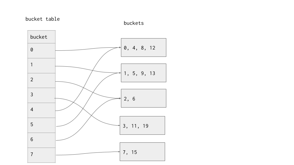
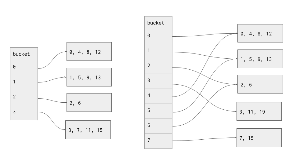
If a bucket overflows and ends up with a local depth greater than the global depth, we need to increase the global depth to maintain a global depth equal to the maximum of the buckets' local depths. To remedy this, we double the size of the hash table by appending it to itself and increasing global depth by 1. Then, we can iterate through and make sure that the buckets are all being pointed to by the correct slots in the hash table. In particular, the bucket that just split should have its slots corrected.
To hammer home this point, consider the following diagram; the left hand side shows the table before the addition of the value "19". As you can see, the hash table was doubled in size, but a new bucket was only made for the bucket index that overflowed.
It is possible that after a split, all of the values in the old bucket ended up in the same bucket, immediately triggering a second split. This can be caused by a bad hash function (imagine a hash function that maps all inputs to the same output), too many duplicates, or due to an adversarial workload. There are many ways to handle recursive splitting, all of which are outside the scope of this chapter.
Other hash-based algorithms such as linear hashing exist. We'll move on to tree-based schemes now, however.
Tree-based Indexing
Tree-based indexing schemes allow for logarithmic-time inserts, updates, and deletions, while also support range questions. In a database, being able to respond with all of the tuples that match a certain range is very useful, which is why the following data structures are used ubiquitously in database systems.
BTrees
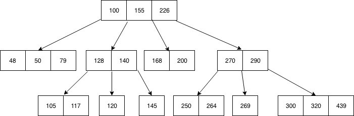
A BTree is a self-balancing recursive data structure that allows logarithmic time search, insertion, and deletion. It is a generalization of the binary search tree in that each node can have more than 1 search key and more than 2 children. A BTree of order \(m\) is formally defined as a tree that satisfies the following properties:
- Each node has at most \(m\) children,
- Every non-leaf (internal) node has at least \(\lceil m/2 \rceil\) children,
- The root has at least two children unless it is a leaf node,
- A non-leaf node with \(k\) children contains \(k-1\) keys,
- All leaves appear on the same level and carry no information.
One way to visualize what an internal node looks like is an array of \(2k-1\) values, alternating between a child node pointer and a key:
[child_1, key_1, child_2, key_2, ..., key_k-1, child_k]
And a leaf node is similarly visualizable, except that there is a one-to-one correspondence between keys and values, making it an array of \(2k\) values:
[key_1, value_1, key_2, value_2, ..., value_k-1, key_k, value_k]
Critically, all of the values of a node in between two values must be between those two values. So, there will never be any keys less than key_1 or greater than key_2 in child_2 or any of its descendants. This mirrors the invariant present in any search tree.
This data structure supports search, insertion, and deletion. Updates are supported as well, but can be thought of as a deletion followed by a subsequent insertion. We describe each of these algorithms.
Search - to search for a entry, we start at the root node. If the entry we're looking for is in this node, we return it. Otherwise, we binary search over the keys to find the branch that our desired entry could be in, and repeat this process for that child node until we either find the entry or bottom out.
Insertion - to insert a entry, we start at the root node. Then, we traverse to a leaf node and insert the entry in the correct spot, assuming the entry doesn't already exist. If the leaf node overflows (i.e. has more than \(k\) entries), then we need to split it so that our BTree is still valid. To split a leaf node, we create a new leaf node and transfer half of the entries (not including the median) over to the new leaf node. Then, we take the median element and push that value up into the parent node to serve as a separator key for our two new nodes. If the parent node overflows, we repeat this process for that node.
Deletion - to delete a value, we first find the value (if it exists), then we remove it. This operation becomes rather complicated when nodes underflow (less than \(\lceil m/2 \rceil\) children), or when deleting a value from an internal node; we leave it as an exercise to the reader to explore this operation.
To explore how some of these BTree operations work, try out this online visualization.
B+Trees
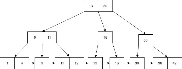
Now that we understand BTrees, it's time to explore what a B+Tree is. A B+Tree is a BTree with a few important changes:
- Each leaf node has a pointer to its right neighbor. This makes linear scans much easier, since we don't have to traverse the tree structure to get to the next leaf node.
- Internal nodes store duplicates of values in leaf nodes. Critically, when a leaf node splits, it doesn't push any entries up to the parent; rather, it only pushes a copy of the entry up. This means that if we were to scan every leaf node, we would retrieve every value in the tree.
Otherwise, everything else is the same as in a BTree. This structure is better optimized for when data you're looking for is on disk, since internal nodes only need to store keys, and then all of the large values are kept on leaf nodes. In our scheme, each node corresponds to a page, meaning the number of pages we have to read in to find a particular value is equal to the height of our B+Tree.
The operations in a B+Tree are slightly different:
Search - to search for a value, we start at the root node and traverse all the way to the correct leaf node, using binary search to descend quickly. Once we arrive at the leaf node, binary search for the value.
Insertion - to insert a value, we start at the root node. Then, we traverse to a leaf node and insert the value in the correct spot. If the leaf node overflows (i.e. has more than \(k\) values), then we need to split it so that our BTree is still valid. To split a leaf node, we create a new leaf node and transfer half of the values (including the median) over to the new leaf node. Then, we take a copy of the median element and push that value up into the parent node to serve as a separator key for our two new nodes. If the parent node overflows, we repeat this process for that node. The main difference here is that we duplicate the median key when we split.
Deletion - to delete a value, we first find the value in a leaf node(if it exists), then we remove it. This operation becomes rather complicated when nodes underflow (less than \(\lceil m/2 \rceil\) children), or when deleting a value from an internal node; we leave it as an exercise to the reader to explore this operation.
To explore how some of these B+Tree operations work, try out this online visualization.
Disk Representation
For both BTrees and B+Trees, each node is typically represented by one page. This means that the number of entries in an internal or leaf node is determines by the page and entry size. Moreover, leaf nodes may contain the row itself if the data is small, but may instead contain the location of the row in data blocks. The former is necessary for secondary indexes.
Node Splitting
Splitting a node is actually quite a tricky operation which requires careful indexing; to help you wrap your head around the implementation of this opereation, we provide the following example. Let's say our internal node looks like this:
[child_0, key_0, child_1, key_1, child_2, key_2, child_3, key_3, child, key_4, child_5]
and then our second child (child index = 1) splits. Here's the node after the split, with child* as the new child, and key* the new key.
[child_0, key_0, child_1, key*, child*, key_1, child_2, key_2, child_3, key_3, child, key_4, child_5]
Notice how many keys and how many children we shifted. We shifted 3 of each. Next, notice the indices of the keys and children that we shifted. We shifted child indexes 3 and above, and we shifted key indexes 2 and above. The indexes for the keys and children we moved do not match up! This subtle nuance can save you a lot of time should you implement this yourself.
Range Queries
One of the B+Tree's biggest optimization is the existence of links between leaf nodes to allow faster linear scans. A cursor is an abstraction that takes advantage of these links to carry out selections quickly.
Essentially, a cursor is a data structure that points to a particular part of another data structure, with a few options for movement and action. A cursor typically has two operations: step and get. stop steps the cursor over the next value; for example, if we are in the middle of a node, it moves on to the next value, otherwise, it skips over to the next node. get returns the value that the cursor is currently pointing at for the surrounding program to handle. Critically, in a B+Tree, a cursor never needs to be in an internal node, making it an easy to understand and simple to use abstraction.
This allows us to easily and abstractly define how a B+Tree can be used to answer a range query. In essense, we first search for the first value that fits in our range, then continually apply the step function, processing each value along the way, until we step out of our range.